AI-Driven Feature Selection in Python!
Deep-dive on ML techniques for feature selection in Python — Part 3
The final part of a series on ML-based feature selection where we discuss advanced methods like Borutapy and Borutashap. Also, discuss how to combine results from multiple methods.
I would like to start by thanking and congratulating the readers who have made it to the final part of this blog series on ML-based feature selection methods!
If you haven’t gone through the first two parts, would request you to kindly go through them:
Deep-dive on ML techniques for feature selection in Python — Part 1
Deep-dive on ML techniques for feature selection in Python — Part 2
We have already covered the following in the previous sections:
A) Types of Feature Selection Methods (Part 1)
B) Correlation: Pearson, Point Bi-Serial, Cramer’s V (Part 1)
C) Weight of Evidence and Information Value (Part 1)
D) Beta Coefficients (Part 2)
E) Lasso Regression (Part 2)
F) Recursive Feature Selection and Sequential Feature Selector (Part 2)
And we will be focusing on the following here:
A)BorutaPy (Part 3)
B) BorutaShap (Part 3)
C) Bringing it all together (Part 3)
As mentioned in earlier parts, the details on the dataset and the entire code (including data preparation) can be found in this Github repo. So let’s dive in!
A) BorutaPy
Boruta made its first appearance in 2010 as a package for R (paper link). It has soon become one of the most popular and advanced methods available for feature selection and it’s based on two concepts:
Concept 1: Shadow features
In Boruta, features are selected based on their performance against a randomized version of them. The main logic is that a feature is useful only if it can perform better than the randomized features. Here are the major steps behind it:
- Based on the original dataframe on the features, another dataframe is generated by randomly shuffling each feature. The permuted features are known as shadow features.
- Then the shadow dataframe is joined with the original one
- Fit the user-defined model on this combined dataframe
- Get importance of all features (original + shadow features)
- Get the highest feature importance recorded among the shadow features (we will call it threshold from now). The python version has a small twist in this step which we will discuss later.
- When the importance of an original feature is higher than this threshold, we call it a “hit”
Taking the maximum of the shadow features as a threshold in selecting features is very conservative at times and hence the python package allows the user to set the percentile of the shadow features’ importances as the threshold. The default of 100 is equivalent to what the R version of Boruta does.
Concept 2:Binomial distribution
The next idea is based on repeating the steps mentioned earlier multiple times to make the results more reliable. If we call each iteration a trial, what is the probability that a feature is selected in a trial? Given we have no clue if a feature is important beforehand, the probability is 50% and since each independent trial can give a binary outcome (hit or no-hit), this series of n trials follow a binomial distribution.
If we plot the binomial probability distribution for 20 trials with 50% success probability and 5% level of significance, the probability curve will look like:
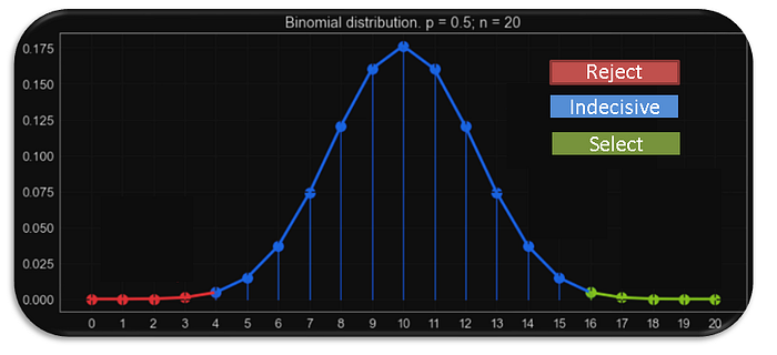
In Borutapy, the features are categorized into 3 parts. The parts are based on the two extreme sections of the distribution called tails (decided by significance level):
- Reject(the red area): The features here are considered noise and should be dropped. In our picture above, if a feature was a hit less than 4 times out of 20 then it’s in this area.
- Indecisive(the blue area): The features here are not conclusive and hence, the model can’t say with confidence to drop/keep. In our picture above, if a feature was a hit less than 16 times and more than 3 times out of 20 then it’s in this area.
- Accept (the green area): The features here are an important estimator. In our picture above, if a feature was a hit more than 15 times out of 20 then it’s in this area.
A detailed example of how BorutaPy is calculated can be found here.
Python implementation of BorutaPy
The python package has some improvements over the R package:
- Faster run times, thanks to scikit-learn
- Scikit-learn like interface
- Compatible with any ensemble method from scikit-learn
- Automatic n_estimator selection
- Ranking of features
- Feature importances are derived from Gini impurity instead of the RandomForest R package’s MDA.
Also, it is highly recommended that we should use pruned trees with a depth between 3–7. Further details on the python package can be found here. The function borutapy_feature_selection allows users to pick from 3 popular tree-based algorithms: XG Boost, Random Forest and Light GBM. The function sets up any estimator from the list specified by the user using the borutapy_estimator parameter. If nothing is mentioned, an XG boost model is fit by default. They can also change a number of other features like the number of trials (see inputs section of the function in the code below).
#7. Select features based on BorutaPy method# BorutaPy:
borutapy_estimator = "XGBoost"
borutapy_trials = 10
borutapy_green_blue = "both"################################ Functions #############################################################def borutapy_feature_selection(data, train_target,borutapy_estimator,borutapy_trials,borutapy_green_blue):

    #Inputs
    # data - Input feature data
    # train_target - Target variable training data
    # borutapy_estimator - base model (default: XG Boost)
    # borutapy_trials -  number of iteration
    # borutapy_green_blue - choice for green and blue features## Initialize borutapy

    if borutapy_estimator == "RandomForest":
        # Manual Change in Parameters - RandomForest
        # Link to function parameters - https://scikit-learn.org/stable/modules/generated/sklearn.ensemble.RandomForestClassifier.html
        estimator_borutapy=RandomForestClassifier(n_jobs = -1,
                                                  random_state=101,
                                                  max_depth=7)
    elif borutapy_estimator == "LightGBM":
        # Manual Change in Parameters - LightGBM
        # Link to function parameters - https://lightgbm.readthedocs.io/en/latest/pythonapi/lightgbm.LGBMClassifier.html
        estimator_borutapy=lgb.LGBMClassifier(n_jobs = -1,
                                              random_state=101,
                                              max_depth=7)
    else:
        # Manual Change in Parameters - XGBoost
        # Link to function parameters - https://xgboost.readthedocs.io/en/stable/parameter.html
        estimator_borutapy = XGBClassifier(n_jobs = -1,
                                           random_state=101,
                                           max_depth=7)## fit Borutapy
    # Manual Change in Parameters - Borutapy
    # Link to function parameters - https://github.com/scikit-learn-contrib/boruta_py
    borutapy = BorutaPy(estimator = estimator_borutapy,
                        n_estimators = 'auto',
                        max_iter = borutapy_trials)
    borutapy.fit(np.array(data), np.array(train_target))

    ## print results
    green_area = data.columns[borutapy.support_].to_list()
    blue_area = data.columns[borutapy.support_weak_].to_list()
    print('features in the green area:', green_area)
    print('features in the blue area:', blue_area)    if borutapy_green_blue == "both":
        borutapy_top_features = green_area + blue_area
    else:
        borutapy_top_features = green_area

    borutapy_top_features_df =pd.DataFrame(borutapy_top_features,
                                           columns = ['Feature'])
    borutapy_top_features_df['Method'] = 'Borutapy'

    return borutapy_top_features_df,borutapy################################ Calculate borutapy #############################################################borutapy_top_features_df,boruta = borutapy_feature_selection(train_features_v2, train_target,borutapy_estimator,borutapy_trials,borutapy_green_blue)borutapy_top_features_df.head(n=20)

B) Boruta SHAP
The Achilles heel of BorutaPy is that it strongly relies on the calculation of the feature importances which can be biased. This is where SHapley Additive exPlanations (SHAP) fits into the puzzle. To keep it simple, SHAP values can explain how a complex model makes its decisions. It essentially calculates the average marginal contributions for each feature across all permutations for each observation. Due to the additive nature of calculations, we can take the average value of these marginal contributions for each observation to achieve global feature importance. A detailed example of how SHAP values are calculated can be found here.
The only con in this method is the evaluation time as there are a number of permutations that need to be calculated.
Python implementation of BorutaShap
The function borutapy_feature_selection allows users to pick from 3 popular tree-based algorithms: XG Boost, Random Forest and Light GBM. The function sets up any estimator from the list specified by the user using the borutapy_estimator parameter. If nothing is mentioned, an XG boost model is fit by default. They can also change a number of other features like the number of trials (see inputs section of the function in the code below).
#8. Select features based on BorutaShap method# BorutaShap:
borutashap_estimator = "XGBoost"
borutashap_trials = 10
borutashap_green_blue = 'both'################################ Functions #############################################################def borutashap_feature_selection(data, train_target,borutashap_estimator,borutashap_trials,borutashap_green_blue):

    #Inputs
    # data - Input feature data
    # train_target - Target variable training data
    # borutashap_estimator - base model (default: XG Boost)
    # borutashap_trials -  number of iteration
    # borutashap_green_blue - choice for green and blue features## Initialize borutashap

    if borutashap_estimator == "RandomForest":
        # Manual Change in Parameters - RandomForest
        # Link to function parameters - https://scikit-learn.org/stable/modules/generated/sklearn.ensemble.RandomForestClassifier.html
        estimator_borutashap=RandomForestClassifier(n_jobs = -1,
                                                    random_state=1,
                                                    max_depth=7)
    elif borutashap_estimator == "LightGBM":
        # Manual Change in Parameters - LightGBM
        # Link to function parameters - https://lightgbm.readthedocs.io/en/latest/pythonapi/lightgbm.LGBMClassifier.html
        estimator_borutashap=lgb.LGBMClassifier(n_jobs = -1,
                                                random_state=101,
                                                max_depth=7)
    else:
        # Manual Change in Parameters - XGBoost
        # Link to function parameters - https://xgboost.readthedocs.io/en/stable/parameter.html
        estimator_borutashap=XGBClassifier(n_jobs = -1,
                                           random_state=101,
                                           max_depth=7)## fit BorutaShap
    # Manual Change in Parameters - BorutaShap
    # Link to function parameters - https://github.com/scikit-learn-contrib/boruta_py
    borutashap = BorutaShap(model = estimator_borutashap,
                            importance_measure = 'shap',
                            classification = True)
    borutashap.fit(X = data, y = train_target,
                   n_trials = borutashap_trials)

    ## print results
    %matplotlib inline
    borutashap.plot(which_features = 'all')## print results
    green_area = borutashap.accepted
    blue_area = borutashap.tentative
    print('features in the green area:', green_area)
    print('features in the blue area:', blue_area)    if borutashap_green_blue == "both":
        borutashap_top_features = green_area + blue_area
    else:
        borutashap_top_features = green_area

    borutashap_top_features_df=pd.DataFrame(borutashap_top_features,
                                            columns = ['Feature'])
    borutashap_top_features_df['Method'] = 'Borutashap'    return borutashap_top_features_df,borutashap################################ Calculate borutashap #############################################################borutashap_top_features_df,borutashap = borutashap_feature_selection(train_features_v2, train_target,borutashap_estimator,borutashap_trials,borutashap_green_blue)
borutashap_top_features_df.head(n=20)

Further details on the python package can be found here.
C) Bringing it all together
Never put all your eggs in one basket
This wise old saying fits perfectly into most applications of data science. More often than not, none of the ML models are free of flaws but each has its own strengths. In my experience, it is always a good strategy to not rely on just one method and use a combination of them if possible. That way we are not susceptible to the major downfalls of any method and leverage the benefits of multiple methods. The same logic can be applied to feature selection techniques. Now that we have learnt 8 different methods, I would suggest the readers use a combination (or all) of them and pick features that were selected by majority of the methods. Here is a quick python code for doing that
# Methods Selectedselected_method = [corr_top_features_df, woe_top_features_df,beta_top_features_df,lasso_top_features_df,
rfe_top_features_df,sfs_top_features_df,borutapy_top_features_df,borutashap_top_features_df]# Combining features from all the models
master_df_feature_selection = pd.concat(selected_method, axis =0)
number_of_methods = len(selected_method)
selection_threshold = int(len(selected_method)/2)
print('Selecting features which are picked by more than ', selection_threshold, ' methods')
master_df_feature_selection_v2 = pd.DataFrame(master_df_feature_selection.groupby('Feature').size()).reset_index()
master_df_feature_selection_v2.columns = ['Features', 'Count_Method']
master_df_feature_selection_v3 = master_df_feature_selection_v2[master_df_feature_selection_v2['Count_Method']>selection_threshold]
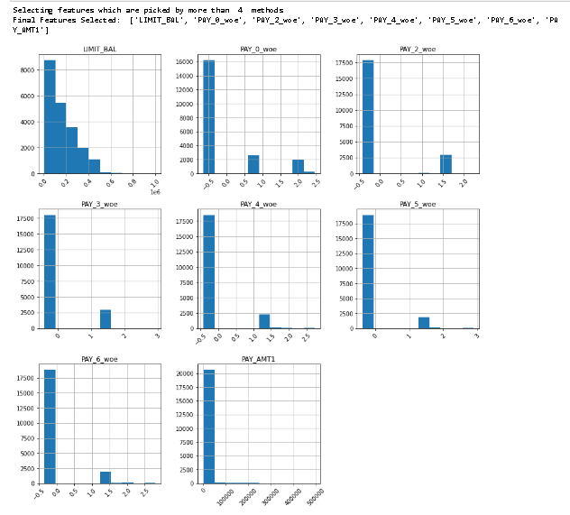
final_features = master_df_feature_selection_v3['Features'].tolist()
print('Final Features Selected: ',final_features)
train_features_v2[final_features].hist(figsize = (14,14), xrot = 45)
plt.show()
master_df_feature_selection_v3.head(n=30)
Final Words
Congratulations!
We have completed the series on ML-based feature selection techniques! We have deep-dived into 8 major methods spread across various categories (filter, wrapper and embedded), computational difficulties and ease of understanding. Not only did we learn the theory behind it but were also able to implement them in python. We also covered the best practices while using them. This blog series along with the reference materials should be enough to get anyone started on using these methods.
The final piece of the puzzle here is to remember that we have only covered the science here but feature selection is an art as well. We will get better at it with practice but I would like to end this series with one piece of advice: Use as many methods as possible and always validate the results based on business logic. Sometimes even if the model is not able to pick some key features but business logic dictates we use it, I would suggest adding it.
Reference Material
Let’s Connect!
If you, like me, are passionate about AI, Data Science or Economics, please feel free to add/follow me on LinkedIn, Github and Medium.
